Ion Exchange Chromatography
Separate proteins by differences in net surface charge, usually with salt or pH elution.
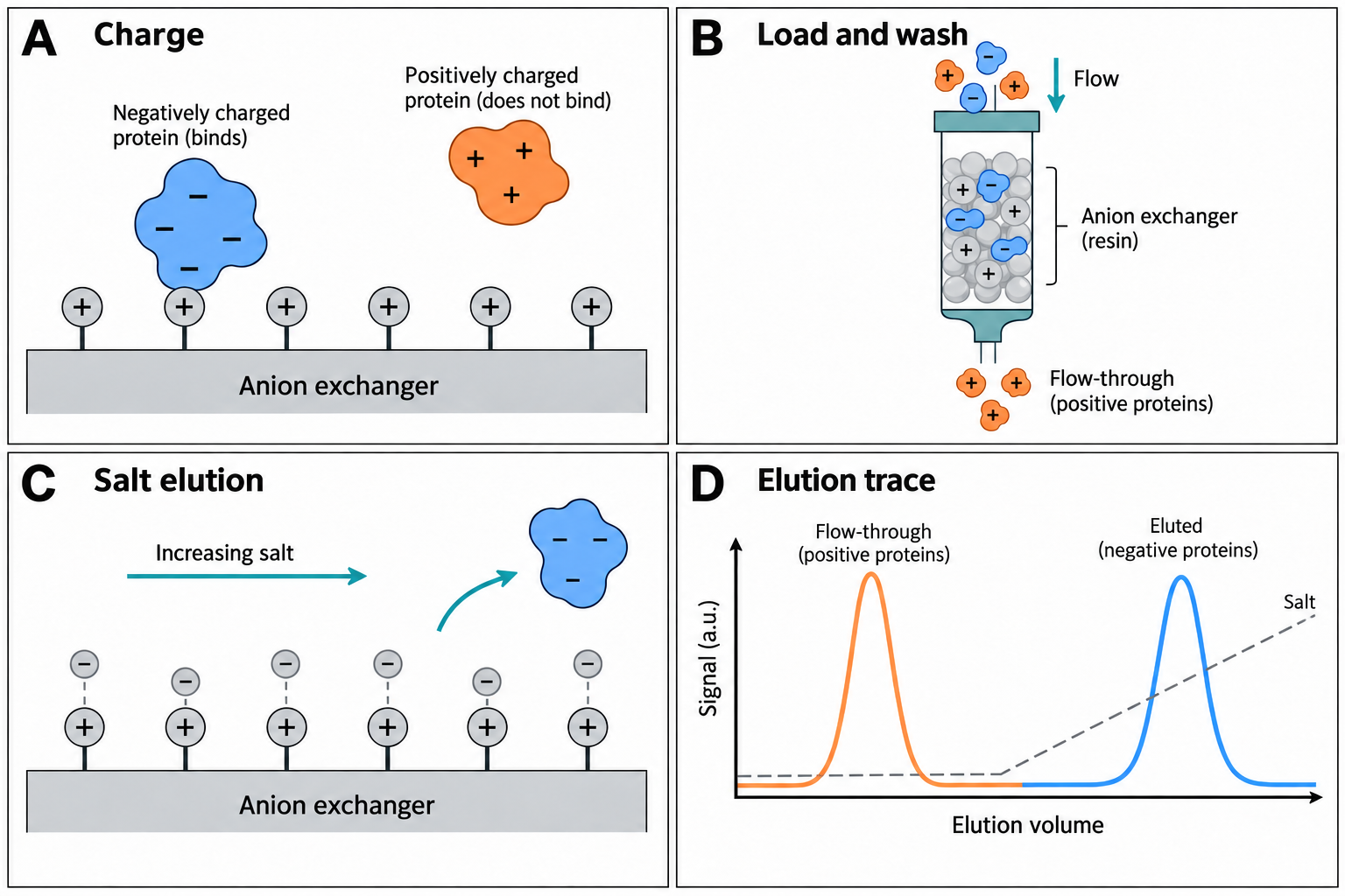
Principle
IEX resins carry fixed charged groups. Proteins bind through electrostatic interaction between charged groups on their surface and the oppositely charged resin. Anion exchangers (for example Q, DEAE) carry positive groups and retain net-negative species; cation exchangers (for example SP, S, CM) carry negative groups and retain net-positive species. Bound proteins are usually eluted by increasing salt concentration, and can also be eluted by changing pH.
Choosing anion vs. cation exchange
As a first approximation, a protein carries a net negative charge above its pI and tends to bind an anion exchanger, and a net positive charge below its pI and tends to bind a cation exchanger. Cytiva™’s IEX handbook suggests a start-buffer pH at least 0.5–1 pH unit from the pI on the appropriate side, and notes that proteins often begin to dissociate about 0.5 pH units from their pI. Binding reflects surface charge and its distribution rather than net charge alone, so retention and elution order cannot be predicted with certainty from the pI. Protein stability over the pH range often decides which exchanger is practical. Conditions can be chosen so that the target binds and many impurities pass through, or the reverse (flowthrough mode); either choice needs experimental confirmation.
Gradient design
- Start buffer: low ionic strength at the chosen pH, with a buffer whose pKa is close to that pH. Confirm the target binds and remains stable.
- Elution buffer: start buffer plus salt (commonly NaCl). A linear gradient of 10–20 CV is a common scouting starting point; the salt range needed is protein- and resin-dependent.
- Shallower gradients can improve resolution between closely related species, at the cost of broader, more dilute peaks.
- Step elution can shorten preparative runs once suitable elution conditions have been established.
Salt-gradient elution in ion exchange
Two illustrative proteins follow the stoichiometric displacement model, k = A·c^(−z), where z is the characteristic charge (the effective number of charges in the binding contact, not the net charge). Change the gradient and watch elution salt, peak width and resolution.
- Protein 1 elutes at
- 246 mM
- Protein 2 elutes at
- 264 mM
- Elution volume 1
- 9.11 CV
- Elution volume 2
- 9.91 CV
- Resolution Rs
- 1.3
- Peak width 2 (4σ)
- 0.61 CV
Model: linear isotherm, unretained salt, zone migration dx/dV = 1/(V0(1+k)) integrated through the column (V0 = 0.4 CV), Gaussian peaks of equal area with σ = V0(1+k at elution)/√N; extra gradient band compression is not applied. Sources: stoichiometric displacement and linear-gradient-elution models as used in Kristl et al., Anal. Chem. 2020 (PMC7307832); gradient trade-offs from the Cytiva™ Ion Exchange Chromatography handbook. Parameters are illustrative, not fitted to a real protein or resin.
Resin types
- Strong exchangers (Q, S, SP) — their ligands stay charged over a broad pH range; protein binding and capacity can still change with pH, conductivity, sample and operating conditions. They are a common starting point for scouting. See experimental pH-dependent capacity on strong exchangers.
- Weak exchangers (DEAE, ANX, CM) — charge and capacity vary with pH; they can offer different selectivity but are more sensitive to pH, flow and load.
- Small-particle media (for example Mono Q, Mono S) — used for high-resolution analytical and polishing work.
Binding capacity, working pH range, flow and pressure limits are specific to each product and are measured under stated conditions. Take them from the current instructions for the exact resin or column.
Troubleshooting IEX
- Target does not bind: check sample and start-buffer pH and conductivity; the sample may need dilution or buffer exchange to lower ionic strength.
- Target appears in the flowthrough: the pH may be on the wrong side of, or too close to, the pI for this exchanger; test the other exchanger type or a different pH.
- Broad or rounded peaks: consider overload, poor packing or channelling, and column contamination; check load, column efficiency and cleaning history.
- Target co-elutes with contaminants: adjust pH, gradient slope or resin chemistry, or add an orthogonal step.
Sources and scope
Cytiva™, Ion Exchange Chromatography: Principles and Methods (official handbook, accessed 2026-09-25) supports the charge/pI relationship and its limits, the 0.5–1 pH unit guidance, strong versus weak exchangers, and the troubleshooting causes above. Its example buffers and gradients are starting points under stated conditions, not universal recipes. Consult the exact resin or column instructions for operating limits.
The charge figure uses the EMBOSS iep pKa set with independent groups. The gradient simulator uses the stoichiometric displacement and linear-gradient-elution models as applied in Kristl et al., Anal. Chem. 2020, with illustrative parameters; it is a teaching model, not a method prediction.
Try it on a trace
Open a two-column chromatogram in the workbench, or load the synthetic example. No account needed.
Open the workbench